Developing a Raycasting ‘3D’ Engine Game in Python and PyGame – PART 1

I have started developing a raycasting game in Python (using PyGame) as a learning exercise and to get a better understanding of the math and techniques involved.

Raycasting is a graphic technique used to render pseudo-3D graphics based on a 2D game world. The best-known example of a raycasting engine used in a computer game is probably Wolfenstein 3D, developed by id Software in 1992.

So firstly, here are some resources I used to upskill and get my head around the topic:

YouTube tutorial series by Standalone Coder. These videos are in Russian, but the YouTube subtitles do a good enough job to follow along.

YouTube tutorial series by Code Monkey King.

Lode’s Computer Graphics Tutorial.

Lastly, I recommend the book Game Engine Black Book: Wolfenstein 3D by Fabien Sanglard, it is not an easy read, but it gives excellent insight into the development of Wolfenstein 3D and a great deal of information into the intricate details of Raycasting and texture mapping.

The Basics of Raycasting

The first thing to understand is that Raycasting is not true 3D, but rather rendering a 2D world in pseudo 3D. Therefore, all movement and game positions consist of only x and y positions, with no height or z positions.

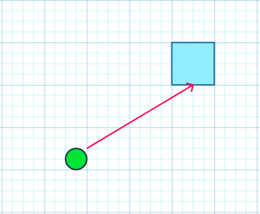
The entire game world consists of a grid, with some blocks in the grid being populated with walls and others being empty. An example of this is shown in the picture below:

In the current version of the game, the world map is implemented as a list of strings, where each character in the string represents a block in the grid. The ‘0’ character represents an empty block, and all other numbers represent a wall. The numbers ‘1’, ‘2’, and ‘3’ are used to show different wall textures according to the different numbers, something covered later in this post.

game_map = [
    '11111111111111111111',
    '10000000000003330001',
    '10011100000000000001',
    '10030000000000000001',
    '10020000000000300001',
    '10020001110000000001',
    '10000330000000000001',
    '10000330000000000001',
    '10000330000000000001',
    '10000330000000000001',
    '10000330000000000001',
    '10000330000000000001',
    '10020000000000300001',
    '10020001110000000001',
    '10000330000000000001',
    '10000330000000000001',
    '10020000000000300001',
    '10020001110000000001',
    '10000330000000000001',
    '11111111111111111111'
]

This is then converted into a dictionary as follows:

world_map = {}
for j, row in enumerate(game_map):
    for i, char in enumerate(row):
        if char != '0':
            if char == '1':
                world_map[(i * GRID_BLOCK, j * GRID_BLOCK)] = '1'
            elif char == '2':
                world_map[(i * GRID_BLOCK, j * GRID_BLOCK)] = '2'
            elif char == '3':
                world_map[(i * GRID_BLOCK, j * GRID_BLOCK)] = '3'

The player is placed on this grid with a x and y coordinates determining the player’s position on the grid. Along with the x and y coordinates, the player also has a viewing angle, i.e., a direction the player is facing.

Now that we have the foundation in place, we can get to the raycasting.

To understand this concept, imagine a line originating from the player and heading off in the direction the player is facing.

Now, this is not an endless line, but rather a line that keeps expanding from one world grid line to the next. (this is done with a for loop).

At every point where this ‘ray’ intersects a grid line on the game world, a check is done to determine if the grid line in question is a wall or not.

If it is a wall, the loop expanding the line is stopped, and the x and y coordinates where the wall was intersected will be noted. We will use this a bit later when drawing the pseudo-3D rendering of the world.

The above is the simplest form of raycasting. However, a single ray will not give us a usable amount of information to do the pseudo-3D render with. This is where a player’s FOV (field of view) and more rays come in.

The Player FOV is an angle on the game world originating at the player and extending out in a triangular form. This determines where the player’s visible range at present begins and ends. For this game, I will use a FOV of 60% (i.e., pi/3).

To change the FOV, the following can be used as a guide:

RadiansDegrees
π / 630°
π / 4 45°
π / 360°
π / 290°
π 180°

Within this FOV, several rays will be generated, exactly as per the single one in the example discussed earlier.

In this game, a value of 480 rays has been defined, which will be generated within the FOV, so the process above for a single ray will be repeated 480 times, with each ray cast having its angle increased by a marginal amount from the previous ray.

The angle of the first ray will be determined as follows:

Starting angle = Player Angle – Half the FOV

Where Player Angle is defined as the center point of direction player is facing.

For each subsequent ray, the angle of the ray will be increased by a delta angle calculated as followed:

Delta Angle = FOV/Number of Rays

This will allow for a sufficient set of information to draw a pseudo-3D rendering from.

To see how this is implemented, please look at lines 6 to 39 in the raycasting.py file.

Sine and Cosine functions are used to determine the intersecting coordinates, and if you require a refresher on these functions, I recommend this web article from mathisfun.com.

For calculating the y coordinate where the ray intersects with a wall, the following formula is used:

y = (player y) + depth * sin(ray angle)

And to calculate the x coordinate where the ray intersects with a wall, the following formula is used:

x = (player x) + depth * cos(ray angle)

For depth value in the above formulas, a sequence of numbers would usually be looped through, starting at 0 and ending at some defined maximum depth.

The above formulas would then be executed at each new depth level to get the corresponding x and y coordinates.

This does provide the desired results, but it is not very optimized.

To improve the performance of this operation, the Digital Differential Analyzer (DDA) algorithm will be used. At a high level, the DDA algorithm functions by not checking every pixel of the 2D game world for an intersection of a ray and a wall but only checking on the grid lines of the 2D world (the only place where walls can occur).

To implement the DDA algorithm, we are going to need four extra variables in conjunction with the Player x and y coordinates, namely:

dx and dy – these two variables will determine the step size to the next grid line. Based on the direction of the angle, these either have the value of 1 or -1.

gx and gy – This will be the x and y coordinates of the grid lines that will be iterated through, starting with the grid line the closest to the player x and y position. The initial value is determined using the following function, located in the common.py file:

def align_grid(x, y):
    return (x // GRID_BLOCK) * GRID_BLOCK, (y // GRID_BLOCK) * GRID_BLOCK

This will ensure that the returned x and y coordinates are located on the closet grid line (based on game world tile size). For reference, the // operator in Python is floor division and rounds the resulting number to the nearest whole number down.

To determine the depth to the next y-axis grid line, the following equation will be used:

Depth Y = (gx – player x) / cos (ray angle)

And to determine the depth of the next x-axis grid line, this equation is used:

Depth X = (gy – player y) / sin (ray angle)

The below two code blocks implement what was just described, the first block of code is to determine intersections with walls on the y axis of the world map:

        # checks for walls on y axis
        gx, dx = (xm + GRID_BLOCK, 1) if cos_a >= 0 else (xm, -1)
        for count in range(0, MAX_DEPTH, GRID_BLOCK):
            depth_y = (gx - px) / cos_a
            y = py + depth_y * sin_a
            tile_y = align_grid(gx + dx, y)
            if tile_y in world_map:
                # Ray has intersection with wall
                texture_y = world_map[tile_y]
                ray_col_y = True
                break
            gx += dx * GRID_BLOCK

And the next block of code is to determine intersections with walls on the x axis of the world map:

        # checks for walls on x axis
        gy, dy = (ym + GRID_BLOCK, 1) if sin_a >= 0 else (ym, -1)
        for count in range(0, MAX_DEPTH, GRID_BLOCK):
            depth_x = (gy - py) / sin_a
            x = px + depth_x * cos_a
            tile_x = align_grid(x, gy + dy)
            if tile_x in world_map:
                # Ray has intersection with wall
                texture_x = world_map[tile_x]
                ray_col_x = True
                break
            gy += dy * GRID_BLOCK

texture_x and texture_y are used to store the index of the texture to display on the wall. We will cover this later in this post.


Now that we have the raycasting portion covered, which is the most complex, we can focus on simply rendering the pseudo-3D graphics to the screen.

At a very high level, the basic concept of how the pseudo-3D graphics will be created, is to draw a rectangle for every ray that has intersected a wall. The x position of the rectangle will be based on the angle of the ray. The y position will be determined based on the distance of the wall from the player, with a width of the rectangle equal to the distance between the rays (calculated with Window resolution width / Number of Rays) and a user-defined height.

This will create a very basic pseudo-3D effect, and it would be much nicer using textured walls.

To implement textured walls the concept remains the same, but instead of just drawing rectangles, we will copy a small strip from a texture image and draw that to the screen instead.

In the code blocks above, there were two variables texture_x and texture_y. Where a wall intersection did occur these variables will contain a value of ‘1’, ‘2’ or ‘3’ based on the value in the world map, and these correspond to different textures that are loaded in a dictionary as follows:

textures = {
                    '1': pygame.image.load('images/textures/1.png').convert(),
                    '2': pygame.image.load('images/textures/2.png').convert(),
                    '3': pygame.image.load('images/textures/3.png').convert(),
                    'S': pygame.image.load('images/textures/sky.png').convert()
                   }

Firstly the correct section of the texture needs to be loaded based on the ray’s position on the wall. This is done as follows:

wall_column = textures[texture].subsurface(offset * TEXTURE_SCALE, 0, TEXTURE_SCALE, TEXTURE_HEIGHT)

Depending if it is for a x-axis or y-axis wall, the follwoing values will be as follows:

For a x-axis wall:

texture = texture_x

offset = int(x) % GRID_BLOCK

Where x is the x coordinate of the wall intersection.

And for a y-axis wall:

texture = texture_y

offset = int(y) % GRID_BLOCK

Where y is the y coordinate of the wall intersection.

Next, the section of the texture needs to be resized correctly based on its distance from the player as follows:

wall_column = pygame.transform.scale(wall_column, (SCALE, projected_height))

Where the values are determined as below:

projected_height = min(int(WALL_HEIGHT / depth), 2 * resY)

resY = Window Resolution Height

For a x-axis wall:

depth = max((depth_x * math.cos(player_angle – cur_angle)),0.00001)


For a y-axis wall:

depth = max((depth_y * math.cos(player_angle – cur_angle)),0.00001)

The last thing to do then is to draw the resized texture portion to the screen:

sc.blit(wall_column, (ray * SCALE, HALF_HEIGHT - projected_height // 2))

The above operations of copying a section of a texture, resizing it, and drawing it to the screen is done for every ray that intersects a wall.

The last thing to do and by far the least complex is to draw in the sky box and the floor. The sky box is simply an image, loaded in the texture dictionary under the ‘S’ key, which is drawn to the screen. The sky box is drawn in three blocks:

        sky_offset = -5 * math.degrees(angle) % resX
        self.screen.blit(self.textures['S'], (sky_offset, 0))
        self.screen.blit(self.textures['S'], (sky_offset - resX, 0))
        self.screen.blit(self.textures['S'], (sky_offset + resX, 0))

This ensures that no gap appears as the player turns and creates the impression of an endless sky.

Lastly, for the floor, a solid color rectangle is drawn as below:

pygame.draw.rect(self.screen, GREY, (0, HALF_HEIGHT, resX, HALF_HEIGHT)) 

For reference, the following PyGame functions are used in the game up to this point:

pygame.init
Used to initialize pygame modules and get them ready to use.

pygame.display.set_mode
Used to initialize a window to display the game.

pygame.image.load
Used to load an image file from the supplied path into a variable to be used when needed.

pygame.Surface.subsurface
Used to get a copy of a section of an image (surface) based on the supplied x position,y position, width, and height values.

pygame.transform.scale
Used to resize an image (surface) to the supplied width and height.

pygame.Surface.blit
Used to draw images to the screen.

pygame.display.flip
Used to update the full display Surface to the screen.

pygame.Surface.fill
Used to fill the display surface with a background color.

pygame.draw.rect
Used to draw a rectangle to the screen (used for the floor).

Also used pygame.key.get_pressed, pygame.event.get and pygame.mouse methods for user input.

Collision Detection

Because the game plays out in a 2D world, collision detection is rather straightforward.

The player has a square hitbox, and every time the player inputs a movement, the check_collision function is called with the new x and y positions the player wants to move to. The function then uses the new x and y positions to determine the player hitbox and check if it is in contact with any walls; if so, the move is not allowed. Otherwise, the player x and y positions are updated to the new positions.

Here is the check_collision function that forms part of the Player class:

 def check_collision(self, new_x, new_y):
        player_location = mapping(new_x , new_y)
        if player_location in world_map:
            #  collision
            print("Center Collision" + str(new_x) + " " + str(new_y))
            return

        player_location = mapping(new_x - HALF_PLAYER_MARGIN, new_y - HALF_PLAYER_MARGIN)
        if player_location in world_map:
            #  collision
            print("Top Left Corner Collision" + str(new_x) + " " + str(new_y))
            return

        player_location = mapping(new_x + HALF_PLAYER_MARGIN, new_y - HALF_PLAYER_MARGIN)
        if player_location in world_map:
            #  collision
            print("Top Right Corner Collision" + str(new_x) + " " + str(new_y))
            return

        player_location = mapping(new_x - HALF_PLAYER_MARGIN, new_y + HALF_PLAYER_MARGIN)
        if player_location in world_map:
            #  collision
            print("Bottom Left Corner Collision" + str(new_x) + " " + str(new_y))
            return

        player_location = mapping(new_x + HALF_PLAYER_MARGIN, new_y + HALF_PLAYER_MARGIN)
        if player_location in world_map:
            #  collision
            print("Bottom Right Corner Collision" + str(new_x) + " " + str(new_y))
            return

        self.x = new_x
        self.y = new_y

Here is a video of the current version of the game in action:

The current version of this game is still a work in progress, but if you are interested, the source code can be downloaded here and the executable here.

Some of the next things on the to-do list are loading levels from the file, adding sprites to the game world, and adding some interactive world items, such as doors that open and close.

I will keep creating posts on this topic as I progress with this project.

Developing a Raycasting ‘3D’ Engine Game in Python and PyGame – PART 1

REVIEW – Audio-Technica ATH-M40x

A few months ago I had to replace my daily driver headphones after my Samson Z55 headphones broke after nearly four years of everyday use (the bracket connecting one of the ear cups snapped off). After doing some research and being unable to source another Samson Z55, I decided on getting the Audio-Technica ATH-M40x.

The ATH-M40x are closed-back dynamic headphones with 40mm rare earth magnet drivers, with an impedance of 35 ohms, making them very easy to power.

The headphones have a frequency response of 15 – 24,000 Hz and are tuned flat for incredibly accurate sound monitoring across the entire frequency range, thus making them excellent studio reference headphones.

The headphone consists of a mainly plastic construction with a folding design, making them easy to pack away in a travel bag.

As with most decent headphones, the ATH-M40x has a detachable cable. The one thing to note is that the cable connects to the headphones via a 2.5mm jack, instead of a 3.5mm jack, as with many headphones.

The ATH-M40x headphones have a very comfortable fit, except for the included ear pads, which I found too small and caused unpleasant pressure on my ears, a common problem I have found with most earpads included with headphones. I resolved this issue by replacing the earpads with the Brainwavz Hybrid Memory Foam Ear Pads, available on Amazon for around $25.

I enjoy the sound quality and tuning of the ATH-M40x, and after a few months of usages, I am impressed by the quality they offer, especially at the $99 price point. Although the ATH-M40x will not be to everyone’s tastes, especially for people who prefer heavier bass, I can highly recommend them for anyone looking for a comfortable neutral headphone.

The Audio-Technica ATH-M40x is available on Amazon for $99.

REVIEW – Audio-Technica ATH-M40x

3D PRINTING REVIEW – FILLAMENTUM PLA EXTRAFILL

Fillamentum is a Czech Republic-based company specializing in the manufacturing of high-quality 3D printing filaments. Their PLA filament, which they call PLA Extrafill. The filament is made of natural ingredients and can be biodegraded by industrial composting. PLA Extrafill is also safe for food contact applications.

Fillamentum PLA Extrafill is more expensive than many other companies PLA filaments, costing approximately $26 (USD) for 750 grams of filament compared to approximately $28 (USD) for 1kg of CCTREE filament.

Extrafill is available in diameters of 1.75 mm and 2.85 mm (with a diameter tolerance of +-0.05mm), and in a wide variety of colors, I used “Traffic Black” for this review.

As with all PLA-based filaments, it has a recommended printing temperature of 190-210°C.

I experienced a great deal of difficulty successfully printing this PLA, far more than any other PLA I have used in the past. The PLA Extrafill kept clogging the 3D printer hot end with every single print. I tried various setting profiles in Cura. However, the result was always a clogged hot end. This was the case until I dropped the default retraction distance in CURA by a third, and this rectified the clogging hot end issue and allowed me to complete a few successful prints. However, reducing the retraction distance did result in a great deal of striking, more than any other PLA I have ever used. I did manage to reduce this by changing the travel and retraction speeds and reducing the print temperature to 180°C.

Here are some photos of my attempts to print the 3DBenchy model. They illustrate nicely the difficulties encountered.

As I kept refining the settings, I managed to get better results and eliminated more of the print issues I experienced.

Here are some pictures of a Judge Dredd bust with only slight drooping issues around the helmet.

I also printed a Desk organizer to store my 3D print finishing tools.

I finally managed to refine my setting to the point where I could print miniatures with a great level of detail.

The Above picture shows the miniatures next to a AA battery for scale.

If anyone is interested in the Cure settings used to print these miniatures, you can download my Cura settings profile here. This was configured on Cura 4.8.0.

Fillamentum PLA Extrafill is capable of producing excellent results if you put in the work. However, I do feel that given the difficulties experienced with the filament and the results being no better than other less expensive filaments, for example, eSun PLA+, I find Fillamentum PLA Extrafill extremely difficult to recommend.

3D PRINTING REVIEW – FILLAMENTUM PLA EXTRAFILL

2021 PROJECTS

In this post, I will cover some projects I have worked on over the last few months and some projects I have planned for the future.

Bipedal Robot


I am currently busy building a bipedal robot based on this Instructables post by K.Biagini. I used his design as a foundation and added additional components and functionality (such as arms and a Piezo for sound).

I had to modify his 3D models to achieve what I wanted. Here are links to download my modified 3d Models:
– Body Extension (to fit in the extra components) – Link
– Modified Head – Link
– Arms – Link

Here is a list of all the electronic components used:
– 1x Arduino Nano
– 6x micro servos
– 2 x push buttons
– 1x mini toggle switch
– 1x 9v Battery
– 1x ultrasonic sensor (HC-SR04)
– 1x RGB LED
– 1x Piezo

These components are connected as follows:

Pinout configuration of Arduino Nano:

Pin NumberConnected Hardware
2Ultrasonic Sensor Echo Pin
3RGB LED Red Pin
4Push Button 1
5RGB LED Green Pin
6RGB LED Blue Pin
7Push Button 2
8Servo Signal Pin (Right Hip)
9Servo Signal Pin (Right Ankle)
10Servo Signal Pin (Left Hip)
11Piezo
12Servo Signal Pin (Left Ankle)
13Ultrasonic Sensor Trigger Pin
14 (A0)Servo Signal Pin (Left Arm)
15 (A1)Servo Signal Pin (Right Arm)

This is still an in-progress project and is not done, Especially from a coding perspective on the Arduino, but once I have completed this project, I will create a post containing the complete source code.

Rotary Control

I needed a rotary control for another project discussed below, so I decided to build one as per this Post on the Prusa Printers blog. It is based on an Arduino Pro Micro and uses Rotary Encoder Module.

I modified the code available on the Prusa blog to mimic keyboard WASD inputs. Turning the dial left and right will input A and D, respectively. Pressing in the dial control push button will switch to up and down inputs, thus turning the dial left and right will input W and S.
Here is the modified code (Based on Prusa Printers blog post code):

#include <ClickEncoder.h>
#include <TimerOne.h>
#include <HID-Project.h>

#define ENCODER_CLK A0 
#define ENCODER_DT A1
#define ENCODER_SW A2

ClickEncoder *encoder; // variable representing the rotary encoder
int16_t last, value; // variables for current and last rotation value
bool upDown = false;
void timerIsr() {
  encoder->service();
}

void setup() {
  Serial.begin(9600); // Opens the serial connection
  Keyboard.begin();
  encoder = new ClickEncoder(ENCODER_DT, ENCODER_CLK, ENCODER_SW); 

  Timer1.initialize(1000); // Initializes the timer
  Timer1.attachInterrupt(timerIsr); 
  last = -1;
} 

void loop() {  
  value += encoder->getValue();

  if (value != last) { 
    if (upDown)
    {
    if(last<value) // Detecting the direction of rotation
        Keyboard.write('s');
      else
        Keyboard.write('w');
    }
    else
    {
      if(last<value) // Detecting the direction of rotation
        Keyboard.write('d');
      else
        Keyboard.write('a');
    }
    last = value; 
    Serial.print("Encoder Value: "); 
    Serial.println(value);
  }

  // This next part handles the rotary encoder BUTTON
  ClickEncoder::Button b = encoder->getButton(); 
  if (b != ClickEncoder::Open) {
    switch (b) {
      case ClickEncoder::Clicked: 
        upDown = !upDown;
      break;      
      
      case ClickEncoder::DoubleClicked: 
        
      break;      
    }
  }

  delay(10); 
}

I use the rotary control with a Raspberry Pi to control a camera pan-tilt mechanism. Here is a video showing it in action:

I will cover the purpose of the camera as well as the configuration and coding related to the pan-tilt mechanism later in this post.

Raspberry Pi Projects

Raspberry Pi and TensorFlow lite

TensorFlow is a deep learning library developed by Google that allows for the easy creation and implementation of Machine Learning models. There are many articles available online on how to do this, so I will not focus on how to do this.

At a high level, I created a basic object identification model created on my windows PC and then converted the model to a TensorFlow lite model that can be run on a Raspberry pi 4. When the TensorFlow lite model is run on the Raspberry Pi, a video feed is shown of the attached Raspberry Pi camera, with green blocks around items that the model has identified with a text label of what the model believes the object is, as well as a numerical percentage which indicates the level of confidence the model has in the object identification.

I have attached a 3inch LCD screen (in a 3D printed housing) to the Raspberry Pi to show the video feed and object identification in real-time.

The Raspberry Pi Camera is mounted on a pan-tilt bracket which is controlled via two micro servos. As mentioned earlier, the pan-tilt mechanism is controlled via the dial control discussed earlier. The pan-tilt mechanism servos are driven by an Arduino Uno R3 connected to the Raspberry Pi 4 via USB. I initially connected servos straight to Raspberry Pi GPIO pins. However, this resulted in servo jitter. After numerous modifications and attempted fixes, I was not happy with the results, so I decided to use an Arduino Uno R3 to drive the servos instead and connect it to the Raspberry Pi Via USB. I have always found hardware interfacing significantly easier with Arduino and also the result more consistent.

Here is a diagram of how the servos are connected to the Arduino Uno R3:

Below is the Arduino source code I wrote to control the servos. Instructions are sent to the Arduino through serial communication via USB, and the servos are adjusted accordingly.

#include <Servo.h>
#define SERVO1_PIN A2
#define SERVO2_PIN A3

Servo servo1;
Servo servo2;
String direction;
String key;
int servo1Pos = 0;
int servo2Pos = 0;

void setup()
{
  servo1Pos = 90;
  servo2Pos = 90;
  Serial.begin(9600);
  servo1.attach(SERVO1_PIN);
  servo2.attach(SERVO2_PIN);

  servo1.write(30);
  delay(500);
  servo1.write(180);
  delay(500);
  servo1.write(servo1Pos);
  delay(500);
  servo2.write(30);
  delay(500);
  servo2.write(150);
  delay(500);
  servo2.write(servo2Pos);
  delay(500);
  Serial.println("Started");
  servo1.detach();
  servo2.detach();
}

String readSerialPort()
{
  String msg = "";
  if (Serial.available()) {
    delay(10);
    msg = Serial.read();
    Serial.flush();
    msg.trim();
    Serial.println(msg);
  }
  return msg;
}

void loop()
{
  direction = "";
  direction = readSerialPort();
  //Serial.print("direction : " + direction);
  key = "";

  if (direction != "")
  {
    direction.trim();
    key = direction;

    servo1.attach(SERVO1_PIN);
    servo2.attach(SERVO2_PIN);

    if (key == "97")
    {
      if (servo2Pos > 30)
      {
        servo2Pos -= 10;
      }
      servo2.write(servo2Pos);
      delay(500);
      Serial.print("A");
    }

    else if (key == "115")
    {
      if (servo1Pos < 180)
      {
        servo1Pos += 10;
      }
      servo1.write(servo1Pos);
      delay(500);
      Serial.print("S");
    }

    else if (key == "119")
    {
      if (servo1Pos > 30)
      {
        servo1Pos -= 10;
      }
      servo1.write(servo1Pos);
      delay(500);
      Serial.print("W");
    }

    else if (key == "100")
    {
      if (servo2Pos < 150)
      {
        servo2Pos += 10;
      }
      servo2.write(servo2Pos);
      delay(500);
      Serial.print("D");
    }

    delay(100);
    servo1.detach();
    servo2.detach();
  }

}

On the Raspberry Pi, the following Python script is used to transfer the rotary control input via serial communication to the Arduino:

# Import libraries
import serial
import time
import keyboard
import pygame

pygame.init()
screen = pygame.display.set_mode((1, 1))

with serial.Serial("/dev/ttyACM0", 9600, timeout=1) as arduino:
    time.sleep(0.1)
if arduino.isOpen():
    done = False
while not done:
    for event in pygame.event.get():
    if event.type == pygame.QUIT:
    done = True
elif event.type == pygame.KEYDOWN:
if event.key == pygame.K_s:
    arduino.write('s'.encode())

if event.key == pygame.K_w:
    arduino.write('w'.encode())

if event.key == pygame.K_a:
    arduino.write('a'.encode())

if event.key == pygame.K_d:
    arduino.write('d'.encode())
time.sleep(0.5)

arduino.Close();
print ("Goodbye")

The next thing I want to implement on this project is face tracking using TensorFlow lite with automated camera movement.

Raspberry Pi Zero W Mini PC

I built a tiny PC using a Raspberry Pi Zero W combined with a RII RT-MWK01 V3 wireless mini keyboard and a 5 inch LCD display for Raspberry Pi with a 3D printed screen stand.


It is possible to run Quake 1 on the Raspberry Pi Zero following the instructions in this GitHub, and it runs great.

Raspberry Pi Mini Server Rack

I have 3D printed a mini server rack and configured a four Raspberry Pi Cluster consisting of three raspberry Pi 3s and one Raspberry Pi 2. They are all networked via a basic five-port switch.

I am currently busy with a few different projects using the Pi cluster and will have some posts in the future going into some more details on these projects.

I developed a little Python application to monitor my different Raspberry Pis and show which ones are online (shown in green) and offline (shown in red).

The application pings each endpoint every 5 seconds, and it is also possible to click on an individual endpoint to ping it immediately. The list of endpoints is read from a CSV file, and it is easy to add additional endpoints. The UI is automatically updated on program startup with the endpoints listed in the CSV file.

Here is the Python source code of the application:

import PySimpleGUI as sg
import csv
import time
import os
from apscheduler.schedulers.background import BackgroundScheduler


def ping(address):
    response = os.system("ping -n 1 " + address)
    return response


def update_element(server):
    global window
    global layout
    response = ping(server.address)
    if response == 0:
        server.status = 1
        window.Element(server.name).Update(button_color=('white', 'green'))
        window.refresh()
    else:
        server.status = 0
        window.Element(server.name).Update(button_color=('white', 'red'))
        window.refresh()


def update_window():
    global serverList
    for server in serverlist:
        update_element(server)


class server:
    def __init__(self, name, address, status):
        self.name = name
        self.address = address
        self.status = status


serverlist = []

with open('servers.csv') as csv_file:
    csv_reader = csv.reader(csv_file, delimiter=',')
    line_count = 0
    for row in csv_reader:
        if line_count == 0:
            line_count += 1
        else:
            serverlist.append(server(row[0], row[1], 0))
            line_count += 1

layout = [
    [sg.Text("Server List:")],
]

for server in serverlist:
    layout.append([sg.Button('%s' % server.name, 
                    button_color=('white', 'orange'), 
                    key='%s' % server.name)])

window = sg.Window(title="KillerRobotics Server Monitor", 
                    layout=layout, margins=(100, 30))
window.finalize()
scheduler = BackgroundScheduler()
scheduler.start()

scheduler.add_job(update_window, 'interval', seconds=5, id='server_check_job')

while True:
    event, values = window.read()
    if event == sg.WIN_CLOSED:
        scheduler.remove_all_jobs()
        scheduler.shutdown()
        window.close()
        break
    elif event in [server.name for server in serverlist]:
        scheduler.pause()
        update_element([server for server in 
                         serverlist if server.name == event][0])
        scheduler.resume()

Raspberry Pi Pico

I ordered a few Raspberry Pi Picos on its release, and thus far, I am very impressed with this small and inexpensive microcontroller.

The Raspberry Pi Pico sells for $4 (USD) and has the following specifications:
– RP2040 microcontroller chip designed by Raspberry Pi
– Dual-core Arm Cortex-M0+ processor, flexible clock running up to 133 MHz
– 264KB on-chip SRAM
– 2MB on-board QSPI Flash
– 26 multifunction GPIO pins, including 3 analogue inputs
– 2 × UART, 2 × SPI controllers, 2 × I2C controllers, 16 × PWM channels
– 1 × USB 1.1 controller and PHY, with host and device support
– 8 × Programmable I/O (PIO) state machines for custom peripheral support
– Low-power sleep and dormant modes
– Accurate on-chip clock
– Temperature sensor
– Accelerated integer and floating-point libraries on-chip

It is a versatile little microcontroller that nicely fills the gap between Arduino and similar microcontrollers and the more traditional Raspberry Pis or similar single board computers.
I have only scratched the surface of using the Pico on some really basic projects, but I have quite a few ideas of using it on some more interesting projects in the future.

3D Printing

I ran into some problems with my 3D printer (Wanhao i3 Mini) over the last few months. The First problem was that half of the printed LCD display died, which was an annoyance, but the printer was still usable. The next issue, which was significantly more severe, was that the printer was unable to heat up the hot end.

My first course of action was to replace both the heating cartridge and the thermistor to ensure that neither of those components were to blame, and unfortunately, they were not. After some diagnostics with a multimeter on the printer’s motherboard, I determined that no power was passing through to the heating cartridge connectors on the motherboard.

I ordered a replacement motherboard and installed it, and the 3D printer is working as good as new again. When I have some more time, I will try and diagnose the exact problem on the old motherboard and repair it.
Here are photos of the old motherboard I removed from the printer:

Below are some photos of a few things I have 3D printed the last few months:

2021 PROJECTS

BOOK REVIEW – NOT ALL FAIRY TALES HAVE HAPPY ENDINGS: THE RISE AND FALL OF SIERRA ON-LINE BY KEN WILLIAMS

Not All Fairy Tales Have Happy Endings, published in 2020, is the memoir written by Ken Williams. He and his wife, Roberta Williams, founded a computer games company in the late 70s that would eventually become Sierra Online, which was for many years one of the largest and best-renowned computer game companies in the world.

The book covers the early years of Ken’s life, including how he met and married Roberta and how she became interested (and some would even say slightly obsessed) with designing computer games. From their first game, Mystery House, that was designed by Roberta and programmed by Ken, to later establishing well-known game series like the King’s Quest, Space Quest, Quest for Glory, and Leisure Suit Larry games, the book provides an insightful and thoroughly entertaining telling of the journey, especially for someone like myself who grew up playing many of these games. The book also has many stories about these games’ now-iconic designers, like Al Lowe (Game designer of, amongst other things, the Leisure Suit Larry games) and Jane Jensen (the person behind the Gabriel Knight series).

Not All Fairy Tales Have Happy Endings tells the story of Sierra Online from creation, through its rise to glory, to its eventual acquisition by CUC International, ultimately leading to its demise.

This book is a must-read for anyone who experienced and enjoyed Sierra games in the 80s and 90s. It is a fantastic read and provides a peek behind the curtain of a company that created games that left a lasting impression on so many. I highly recommended Not All Fairy Tales Have Happy Endings.

BOOK REVIEW – NOT ALL FAIRY TALES HAVE HAPPY ENDINGS: THE RISE AND FALL OF SIERRA ON-LINE BY KEN WILLIAMS

REVIEW – AMAZON KINDLE 2019 MODEL (10TH GENERATION)

The main improvement offered by the 10th generation base model Kindle over its predecessors, is the inclusion of an integrated light, which was previously only a feature of the more expensive Kindle Paperwhite and Kindle Oasis, and this is a game-changer. The inclusion of the light vastly increases the ease by which you can read the Kindle in various conditions and dramatically improves screen visibility.  

While on the topic of the screen, it is Amazon’s 6″ e-Ink glare-free display, with a PPI of 167 pixels per inch and offers a 16-level grayscale color palette, meaning even comic books and graphic novels are easily readable and details do not get lost.

The Kindle 2019 model offers a comfortable read, with text size easily resizable to user taste and allows for much quicker reading.

The Kindle supports books, comics books\graphic novels, magazines, and audiobooks across the following file formats: Kindle Format 8 (AZW3), Kindle (AZW), TXT, PDF, unprotected MOBI, PRC natively; HTML DOC, DOCX, JPEG, GIF, PNG, PMP through conversion; Audible audio format (AAX). Amazon has also vastly improved PDF support, and reading PDFs is now far less painful than in the past.

The Kindle model reviewed here comes with 8GB of non-expandable storage, enough to hold ample books and comics. However, heavy audiobook listeners might want to look at the 32GB version of the Kindle Paperwhite or Kindle Oasis instead.

A Bluetooth audio device is required (Headphone, Speaker, etc.) to listen to audiobooks, and the Kindle does allow the user to switch between reading and listening rather seamlessly.

The Kindle is entirely Wi-Fi enabled, and once online, it seamlessly integrates into the Amazon ecosystem.

Amazon claims a battery life of up to 4-weeks, obviously depending on usage and light brightness selected. I found the Kindle needed to be charged once every ten days or so with moderate usage (1-2 hours a day), and the light turned up to roughly 80% brightness.

The Kindle weighs in at 174g without a cover, making it shockingly light for its size, definitely contributing to its reading comfort.

The Kindle 2019 model retails on Amazon for $89.99 with the special offer enabled (ads show on the device lock screen) and $109.99 without the special offer. I find the special offer unintrusive, especially if you use a cover that obstructs the screen when not in use.

Amazon’s Kindle e-book readers are pretty much the de facto standard for e-book readers, with Amazon controlling over 80% of the e-book reader market, and it is easy to see why. From the ease of use to simple convenience, Amazons Kindle Devices and Ecosystems are hard to beat.    

REVIEW – AMAZON KINDLE 2019 MODEL (10TH GENERATION)

BOOK REVIEW – ZERO TO MAKER: LEARN (JUST ENOUGH) TO MAKE (JUST ABOUT) ANYTHING BY DAVID LANG

Zero to Maker (originally published in 2013) chronicles David Lang’s journey into the Maker movement and documents the learnings and many of the experiences he had along his journey.

David Lang is one of the founders of OpenROV, a low-cost remote-controlled underwater robot, and his journey of becoming a maker is tightly intertwined with this project.

As part of his journey, he visits numerous maker spaces such as Haxlr8r, Maker Faire, Noisebridge, TechSoup, and FabLabs, and explores the topic of gaining access to tools and skills through these spaces.

The book also covers a wide variety of other topics, from the new world of collaborative making and Do-It-Together to Digital Fabrication Techniques such as CAD, 3D Printing, and Laser Cutting. Another interesting subject covered is turning maker projects into businesses and the numerous challenges faced during that process. Possible ways of overcoming these challenges, such as funding your undertaking using a crowdfunding platform such as Kickstarter to how to handle larger batch manufacturing by leveraging maker spaces and their community of makers, are also examined.

The last chapter focuses on educating future generations on the skills and mindset involved in making as well as the numerous benefits associated therewith. Many great initiatives currently underway at numerous schools and other institutions teaching children how to make is covered, and it is a very inspiring read.

The book is a fascinating read that gives some good insight into the maker movement at a high level.  However, It does not provide detailed instructions on any of the skills explored, and if that is your expectation coming in, you will leave disappointed. I recommend Zero to Maker as a light, informative read and found it a pleasant way of spending a few afternoons.

BOOK REVIEW – ZERO TO MAKER: LEARN (JUST ENOUGH) TO MAKE (JUST ABOUT) ANYTHING BY DAVID LANG

REVIEW – COOLER MASTER MM710 PRO-GRADE GAMING MOUSE WITH HONEYCOMB SHELL AND ULTRAWEAVE CABLE

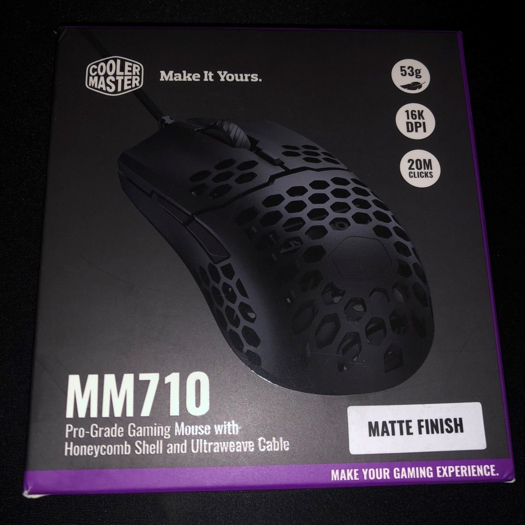
The Cooler Master MM710 is an ultra-light gaming mouse in the same vein of the now famous Glorious Model O mouse. It is currently listed on Amazon at around the $50 price-point, making it a fair bit less expensive than the Glorious Model O. It weighs 53 grams and as someone who usually prefers a heavier mouse, it feels completely weightless.
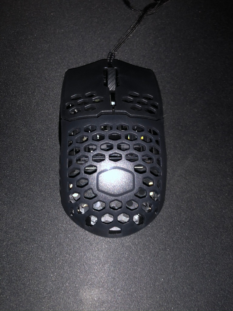
The Honeycomb shell has a very comfortable ergonomic shape, and the ultraweave cable combined with its ultra smooth PTFE feet makes using the mouse absolutely effortless.

The mouse pictured below is the matte black option, however, matte white, gloss black and gloss white options are also available.

Here is a technical specification breakdown of the MM710:

MM710
Year Released 2019
DPI 16000dpi
Buttons 6
Connectivity Wired USB
Weight 53g
Sensor Pixart Optical
Additional Features

Ultra-Lightweight

Ultraweave cable

Omron Switches

The MM710 was the first ultra-lightweight gaming mouse I have tried, and I found using it very comfortable and precise, saying that I am not quite ready to give up the Logitech G603 as my daily driver as I still find it more comfortable. A large part of this relates to the muscle memory I have developed by using a heavier mouse for many years now, and it will take time to get used to such a lightweight mouse.
The MM710 is an excellent product at a very reasonable price, and it is worth considering if you are looking for a lightweight mouse.

REVIEW – COOLER MASTER MM710 PRO-GRADE GAMING MOUSE WITH HONEYCOMB SHELL AND ULTRAWEAVE CABLE

3D PRINT FINISHING

When a 3D print completes printing, it seldom looks like a refined and finished item, from support material that needs to be removed to rough edges that need to be smoothed, quite a bit of work is required to make a 3D print look acceptable.

Here is a quick guide of how I finish my 3D prints to look less like 3D printed items and more like professionally produced commercial products.

Let us first look at the tools I use in the finishing process:

IMG_1747

Wire Cutting Pliers and Long Nose Pliers – These are useful when removing support material from 3D prints.

IMG_1757

Wire Brushes – Perfect for a first pass cleanup on newly printed items to remove any stringing and excess material.

IMG_1754

Needle Files – Useful for smoothing rough spots on prints, especially in small confined areas.

IMG_1761

Craft Knives – To remove any stubborn unwanted material from 3D prints.

IMG_1765

Model Sanding Block – For standing confined areas of 3D prints.

IMG_1770

Heated 3D Print Finishing Tool – Perfect for removing stringing and extra material from 3D prints.

IMG_1782

Sand Paper – Used for general smoothing of 3D prints. It is best to wet sand 3D prints as it prevents the print from melting and getting ruined by the heat created from sanding friction.

IMG_1775

Wood Filler – Used to fill any unwanted gaps and holes in 3D prints.

IMG_1793

Spray Paint Primer – This is used to prime 3D prints for painting. Priming also hides small imperfections on 3D prints. Use a primer that is plastic friendly.

IMG_1779

Model Paint and Brushes – I like Tamiya model paint and brushes, but any model paint supplies should work great.

Now let us look at the finishing process.

Step 1: Select a model and 3D print it.

It is very important to note that the better your 3D printer is maintained and configured, the better the end results will be. Here is an example of the same model 3D printed and finished. The first was printed before I replaced my hot end and did some basic maintenance on my 3D printer (the nozzle was worn, and the heater cartridge started giving issues, I also tightened the belts). The second was printed after I completed the replacement and maintenance.

IMG_1691

The print lines in the first print are clearly visible, even after sanding, while the second model has a smooth finish even with minimal sanding.

Step 2: Remove support material, initial sanding, and filler.

Using wire brushes to do a quick pass over the 3D print to remove any excess material, then sand model using wet sanding method (using sandpaper and water). When sanding the 3D print, start standing with coarse-grit sandpaper (60 grit) and work down to a finer grit (220 grit). Finally, fill any gaps using wood filler.

Step 3: Final Sanding.

When the wood filler has dried, go over the print one final time with very fine grit sandpaper (400 grit).

Step 4: Priming the 3D print

When spraying the 3D print with primer, it is important to hold the spray can at least 30cm away from the 3D print and do long even passes over the model, starting and ending each pass to the side of the 3D print and not directly on the print as it will result in droplets forming.

Step 5: Painting the 3D print

IMG_1601

After the primer has completely dried, it is time to paint the model as desired. Using a wethering technique like black-washing brings out the detail of 3d prints amazingly. Black-washing is done by mixing black (or dark color) paint with some paint thinners, then painting all over the model, putting particular focus on getting the paint into all the nooks and crannies on the print. Then finally wiping away most of the paint with some paper towel. This gives the model a weathered realistic look.

Step 6: Done!

And finally, display your newly created item with pride.

3D PRINT FINISHING

MOVIE REVIEW – MAKER: A DOCUMENTARY ON THE MAKER MOVEMENT

MakerMovie

Maker is a documentary film directed by Mu-Ming Tsai that focuses on the maker movement and the wide variety of topics it entails, such as 3D printing, electronics, biotech, etc.

Numerous interviews with different individuals within the movement are shown and clearly shows the passion they all have. And the film really presses the message across of getting people away from being consumers and becoming makers.

Throughout the documentary, the filmmakers visit various maker spaces and even one biotechnology maker space, and it very interesting to see the facilities on offer.

Two companies formed out of the maker movement, Pebble smartwatches, and OpenROV are also visited, and both illustrate how it is possible to establish companies on the principles of the maker movement.

The film also examines Crowdfunding and how it can provide the financial means for anyone to turn their creations into a consumer product and a successful company.
As an avid supporter of the maker movement, I thoroughly enjoyed the film, and it is an excellent mechanism to introduce people to what the maker movement is. I highly recommend this film.

MOVIE REVIEW – MAKER: A DOCUMENTARY ON THE MAKER MOVEMENT